Wednesday 14 October 2015

radarchart - 'fmsb' package


radarchart() in 'fmsb' package offer a plotting function that draws radar/spider chart, similar to stars() in base package.


library(fmsb) 

'zoo' package converts date values to year-month values.
 
library(zoo) 
 
dat<-as.data.frame(sunspot.month) 

dat$TS<-seq(as.yearmon("1749-01-01"), as.yearmon("2013-09-01"), by = 1/12)
colnames(dat)[1] <- "sunspot"


The decades and centuries were derived from the year-month field to be used for grouping variables as below.

dat$decade <- floor(as.numeric(format(dat$TS, "%Y"))/10)*10
dat$century <- floor(as.numeric(format(dat$TS, "%Y"))/100)*100
dat$month <- format(dat$TS, "%b")
dat$month <- factor(dat$month, levels = unique(dat$month))
  
 
I used 'reshape2' package to rearrange the data to the desired structure while doing the aggregation to obtain mean values.

library(reshape2) 

agg <- recast(data = dat,century~month, measure.var = "sunspot", mean)


radarchart() requires the input data to have the max value and min value in the first and second rows respectively.
  
MX <- c(NA, rep(max(agg[,-1]), ncol(agg)-1)) 
MN <- c(NA, rep(min(agg[,-1]), ncol(agg)-1)) 

agg <- rbind(MX, MN, agg)


To draw a radar chart:

radarchart(agg[,-1])


To assign colours for different groups and to insert a legend:


COL<-colorRampPalette(c("red", "blue"))(nrow(agg)-2) 

radarchart(agg[,-1], pcol = COL) 
legend(2, 1, legend = levels(as.factor(agg$century)), title = "century", col = COL, seg.len = 2, border = "transparent", pch = 16, lty = 1)


To change the line colour in the background:


radarchart(agg[,-1], pcol = COL, cglcol = "grey80") 
legend(2, 1, legend = levels(as.factor(agg$century)), title = "century", col = COL, seg.len = 2, border = "transparent", pch = 16, lty = 1)


To modify number of layers in the background (in this example from 5 to 10):

radarchart(agg[,-1], pcol = COL, cglcol = "grey80", seg = 10) 
legend(2, 1, legend = levels(as.factor(agg$century)), title = "century", col = COL, seg.len = 2, border = "transparent", pch = 16, lty = 1)


To add a title:

radarchart(agg[,-1], pcol = COL, cglcol = "grey80", seg = 10, title = "sun spots") 
legend(2, 1, legend = levels(as.factor(agg$century)), title = "century", col = COL, seg.len = 2, border = "transparent", pch = 16, lty = 1)


To split the groups in to individual radar chart:


par(mfrow = c(2, 2)) 
for(i in 3:nrow(agg)){ 
radarchart(agg[c(1,2,i), -1], pcol = COL[i-2], cglcol = "grey80", seg = 10, title = paste("Century:", agg$century[i], sep=" ")) 
}


To colour the regions/polygons of the above graphs:


par(mfrow=c(2, 2)) 
for(i in 3:nrow(agg)){ 
radarchart(agg[c(1, 2, i), -1], pcol = COL[i-2], cglcol = "grey80", seg = 10, title = paste("Century:", agg$century[i], sep=" "), pdensity = 20, pangle = 30, pfcol = COL[i-2]) 
}


3D Graph - Lattice Package


cloud() function in 'lattice' package provides 3-dimensional visualisation option

library(lattice)

cloud(Sepal.Length~Sepal.Width*Petal.Length,iris,pch=16,alpha=0.7,cex=1,groups=iris$Species)


Adding a title
  
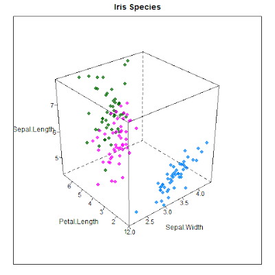
cloud(Sepal.Length~Sepal.Width*Petal.Length,iris,pch=16,alpha=0.7,cex=1,groups=iris$Species,main="Iris Species")  


Modify axis  
  
cloud(Sepal.Length~Sepal.Width*Petal.Length,iris,pch=16,alpha=0.7,cex=1,groups=iris$Species,main="Iris Species",scales=list(arrows=FALSE,x=list(cex=0.9,tck=0.5),y=list(cex=0.9,tck=0.5),z=list(cex=0.9,tck=0.5)))


Modify frame style  
  
cloud(Sepal.Length~Sepal.Width*Petal.Length,iris,pch=16,alpha=0.7,cex=1,groups=iris$Species,main="Iris Species",scales=list(arrows=FALSE,x=list(cex=0.9,tck=0.5,col="wheat3"),y=list(cex=0.9,tck=0.5,col="wheat3"),z=list(cex=0.9,tck=0.5,col="wheat3")),par.settings=list(box.3d=list(col="wheat1")))


Modify axis labels  
  
cloud(Sepal.Length~Sepal.Width*Petal.Length,iris,pch=16,alpha=0.7,cex=1,groups=iris$Species,main="Iris Species",scales=list(arrows=FALSE,x=list(cex=0.9,tck=0.5,col="wheat3"),y=list(cex=0.9,tck=0.5,col="wheat3"),z=list(cex=0.9,tck=0.5,col="wheat3")),par.settings=list(box.3d=list(col="wheat1"),par.xlab.text=list(cex=0.8,col="tan3"),par.ylab.text=list(cex=0.8,col="tan3"),par.zlab.text=list(cex=0.8,col="tan3",rot=90)))


Modify plotting style  
  
cloud(Sepal.Length~Sepal.Width*Petal.Length,iris,pch=16,alpha=0.7,cex=1,groups=iris$Species,main="Iris Species",scales=list(arrows=FALSE,x=list(cex=0.9,tck=0.5,col="wheat3"),y=list(cex=0.9,tck=0.5,col="wheat3"),z=list(cex=0.9,tck=0.5,col="wheat3")),par.settings=list(box.3d=list(col="wheat1"),par.xlab.text=list(cex=0.8,col="tan3"),par.ylab.text=list(cex=0.8,col="tan3"),par.zlab.text=list(cex=0.8,col="tan3",rot=90)),col=c("tan","goldenrod","brown"))


Insert legend/key  
  
cloud(Sepal.Length~Sepal.Width*Petal.Length,iris,pch=16,alpha=0.7,cex=1,groups=iris$Species,main="Iris Species",scales=list(arrows=FALSE,x=list(cex=0.9,tck=0.5,col="wheat3"),y=list(cex=0.9,tck=0.5,col="wheat3"),z=list(cex=0.9,tck=0.5,col="wheat3")),par.settings=list(box.3d=list(col="wheat1"),par.xlab.text=list(cex=0.8,col="tan3"),par.ylab.text=list(cex=0.8,col="tan3"),par.zlab.text=list(cex=0.8,col="tan3",rot=90)),col=c("tan","goldenrod","brown"),key=list(space="right",title="Species",cex.title=1,points=list(col=c("tan","goldenrod","brown"),cex=0.9,pch=16),text=list(lab=levels(iris$Species),cex=0.9)))


Rotating the graph (displayed using 'gridExtra' package for better comparison):
  
library(gridExtra)  
    
- around x-axis  
#default g1<-cloud(Sepal.Length~Sepal.Width*Petal.Length,iris,pch=16,alpha=0.7,cex=1,groups=iris$Species,main="x = -60 (default)",scales=list(arrows=FALSE,x=list(cex=0.9,tck=0.5,col="wheat3"),y=list(cex=0.9,tck=0.5,col="wheat3"),z=list(cex=0.9,tck=0.5,col="wheat3")),par.settings=list(box.3d=list(col="wheat1"),par.xlab.text=list(cex=0.8,col="tan3"),par.ylab.text=list(cex=0.8,col="tan3"),par.zlab.text=list(cex=0.8,col="tan3",rot=90)),col=c("tan","goldenrod","brown"),screen=list(z=40,x=-60,y=0))

#x rotates graph around x axis - i.e. moves viewing  angle up and down - e.g. for view from top (x=0) g2<-cloud(Sepal.Length~Sepal.Width*Petal.Length,iris,pch=16,alpha=0.7,cex=1,groups=iris$Species,main="x = 0",scales=list(arrows=FALSE,x=list(cex=0.9,tck=0.5,col="wheat3"),y=list(cex=0.9,tck=0.5,col="wheat3"),z=list(cex=0.9,tck=0.5,col="wheat3")),par.settings=list(box.3d=list(col="wheat1"),par.xlab.text=list(cex=0.8,col="tan3"),par.ylab.text=list(cex=0.8,col="tan3"),par.zlab.text=list(cex=0.8,col="tan3",rot=90)),col=c("tan","goldenrod","brown"),screen=list(z=40,x=0,y=0))

g3<-cloud(Sepal.Length~Sepal.Width*Petal.Length,iris,pch=16,alpha=0.7,cex=1,groups=iris$Species,main="x = -30",scales=list(arrows=FALSE,x=list(cex=0.9,tck=0.5,col="wheat3"),y=list(cex=0.9,tck=0.5,col="wheat3"),z=list(cex=0.9,tck=0.5,col="wheat3")),par.settings=list(box.3d=list(col="wheat1"),par.xlab.text=list(cex=0.8,col="tan3"),par.ylab.text=list(cex=0.8,col="tan3"),par.zlab.text=list(cex=0.8,col="tan3",rot=90)),col=c("tan","goldenrod","brown"),screen=list(z=40,x=-30,y=0))


grid.arrange(g1,g3,g2,nrow=1,main="Rotating Around X-Axis")


- around z-axis  
  
#z rotates graph around z axis - i.e. moves viewing  angle left and right - e.g. for view from front (z=0) 
g1<-cloud(Sepal.Length~Sepal.Width*Petal.Length,iris,pch=16,alpha=0.7,cex=1,groups=iris$Species,main="z = 40 (default)",scales=list(arrows=FALSE,x=list(cex=0.9,tck=0.5,col="wheat3"),y=list(cex=0.9,tck=0.5,col="wheat3"),z=list(cex=0.9,tck=0.5,col="wheat3")),par.settings=list(box.3d=list(col="wheat1"),par.xlab.text=list(cex=0.8,col="tan3"),par.ylab.text=list(cex=0.8,col="tan3"),par.zlab.text=list(cex=0.8,col="tan3",rot=90)),col=c("tan","goldenrod","brown"),screen=list(z=40,x=-60,y=0))

g2<-cloud(Sepal.Length~Sepal.Width*Petal.Length,iris,pch=16,alpha=0.7,cex=1,groups=iris$Species,main="z = 20",scales=list(arrows=FALSE,x=list(cex=0.9,tck=0.5,col="wheat3"),y=list(cex=0.9,tck=0.5,col="wheat3"),z=list(cex=0.9,tck=0.5,col="wheat3")),par.settings=list(box.3d=list(col="wheat1"),par.xlab.text=list(cex=0.8,col="tan3"),par.ylab.text=list(cex=0.8,col="tan3"),par.zlab.text=list(cex=0.8,col="tan3",rot=90)),col=c("tan","goldenrod","brown"),screen=list(z=20,x=-60,y=0))

g3<-cloud(Sepal.Length~Sepal.Width*Petal.Length,iris,pch=16,alpha=0.7,cex=1,groups=iris$Species,main="z = 0",scales=list(arrows=FALSE,x=list(cex=0.9,tck=0.5,col="wheat3"),y=list(cex=0.9,tck=0.5,col="wheat3"),z=list(cex=0.9,tck=0.5,col="wheat3")),par.settings=list(box.3d=list(col="wheat1"),par.xlab.text=list(cex=0.8,col="tan3"),par.ylab.text=list(cex=0.8,col="tan3"),par.zlab.text=list(cex=0.8,col="tan3",rot=90)),col=c("tan","goldenrod","brown"),screen=list(z=0,x=-60,y=0))

grid.arrange(g1,g2,g3,nrow=1,main="Rotating Around Z-Axis")


- around y-axis  
  
#y rotates graph around y axis - i.e. moves viewing  angle up and down but hinges on y-axisg1<-cloud(Sepal.Length~Sepal.Width*Petal.Length,iris,pch=16,alpha=0.7,cex=1,groups=iris$Species,main="y = 0 (default)",scales=list(arrows=FALSE,x=list(cex=0.9,tck=0.5,col="wheat3"),y=list(cex=0.9,tck=0.5,col="wheat3"),z=list(cex=0.9,tck=0.5,col="wheat3")),par.settings=list(box.3d=list(col="wheat1"),par.xlab.text=list(cex=0.8,col="tan3"),par.ylab.text=list(cex=0.8,col="tan3"),par.zlab.text=list(cex=0.8,col="tan3",rot=90)),col=c("tan","goldenrod","brown"),screen=list(z=40,x=0,y=0))

g2<-cloud(Sepal.Length~Sepal.Width*Petal.Length,iris,pch=16,alpha=0.7,cex=1,groups=iris$Species,main="y = 30",scales=list(arrows=FALSE,x=list(cex=0.9,tck=0.5,col="wheat3"),y=list(cex=0.9,tck=0.5,col="wheat3"),z=list(cex=0.9,tck=0.5,col="wheat3")),par.settings=list(box.3d=list(col="wheat1"),par.xlab.text=list(cex=0.8,col="tan3"),par.ylab.text=list(cex=0.8,col="tan3"),par.zlab.text=list(cex=0.8,col="tan3",rot=90)),col=c("tan","goldenrod","brown"),screen=list(z=40,x=0,y=30))

g3<-cloud(Sepal.Length~Sepal.Width*Petal.Length,iris,pch=16,alpha=0.7,cex=1,groups=iris$Species,main="y = 60",scales=list(arrows=FALSE,x=list(cex=0.9,tck=0.5,col="wheat3"),y=list(cex=0.9,tck=0.5,col="wheat3"),z=list(cex=0.9,tck=0.5,col="wheat3")),par.settings=list(box.3d=list(col="wheat1"),par.xlab.text=list(cex=0.8,col="tan3"),par.ylab.text=list(cex=0.8,col="tan3"),par.zlab.text=list(cex=0.8,col="tan3",rot=90)),col=c("tan","goldenrod","brown"),screen=list(z=40,x=0,y=60))

grid.arrange(g1,g2,g3,nrow=1,main="Rotating Around Y-Axis")


For 3D-bar/column chart:


library(latticeExtra)

Dat <- aggregate(Sepal.Length~Species+Petal.Length, iris, mean)

cloud(Sepal.Length ~ Species + Petal.Length, Dat, panel.3d.cloud = panel.3dbars,
               col.facet=colorRampPalette(c("dodgerblue", "salmon"))(nrow(Dat)),
                xbase = 0.4, ybase = 0.4, scales = list(arrows = FALSE, col = 1),
                col = "white", par.settings = list(axis.line = list(col = "transparent"))
        )


Friday 18 September 2015

alarms, beeps and voice

The below is available in R's base package as a notification method, for example, to alert users that a long running script has finished.

alarm()


'beepr' package is available to provide more options for notification sounds

install.packages("beepr")
library(beepr)
beep()
beep(1)
beep(2)
beep(3)
.
.
.


In Mac, text to speech technique can be called from R

system("say Loop 1 completed")


for different voice options

system("say -v Tessa Loop 2 completed")


Wednesday 22 July 2015

reshape2 package - similar function to pivot table in Excel


recast() in "reshape2" package offers a function that can work like a pivot table in Excel.


library(reshape2)
recast(data = CO2, Plant + Type ~ Treatment, measure.var = "uptake", sum)
   Plant        Type nonchilled chilled
1    Qn1      Quebec      232.6     0.0
2    Qn2      Quebec      246.1     0.0
3    Qn3      Quebec      263.3     0.0
4    Qc1      Quebec        0.0   209.8
5    Qc3      Quebec        0.0   228.1
6    Qc2      Quebec        0.0   228.9
7    Mn3 Mississippi      168.8     0.0
8    Mn2 Mississippi      191.4     0.0
9    Mn1 Mississippi      184.8     0.0
10   Mc2 Mississippi        0.0    85.0
11   Mc3 Mississippi        0.0   121.1
12   Mc1 Mississippi        0.0   126.0


Sometimes, the variables need to be treated as vector.

recast(data=CO2, CO2$Plant + CO2$Type ~ CO2$Treatment, measure.var = "uptake", sum)

Tuesday 7 July 2015

connecting R to database


There are several ways to do this, but the following are what worked for me.


Connections 


Connecting to a database using ODBC:

N.B. 32-bit ODBC will only work with 32-bit R, so for 64-bit R, 64-bit ODBC needs to be installed

library(RODBC)
  
con <- odbcConnect(dsn = "database server name as recorded in ODBC", uid = username, pwd = password) 

N.B For Microsoft SQL Server, I have been told to use odbcDriverConnect instead of odbcConnect.
  
Connecting to Teradata database using JDBC:

library(RJDBC)

drv <- JDBC("com.teradata.jdbc.TeraDriver", "C:/your path to jar file/terajdbc4.jar; C:/
your path to jar file/tdgssconfig.jar") 
con <- dbConnect(drv, "jdbc:teradata://host ip details e.g. 000.00.000.00/", user = "username", password = "password", port = port e.g. 00)  


Connecting to Oracle database:

library(ROracle)

drv <- dbDriver("Oracle")
   
con <- dbConnect(drv, "username", "password", dbname="(DESCRIPTION=(ADDRESS=(PROTOCOL=tcp)(HOST=host ip details e.g. 000.000.0.000)(PORT= port e.g. 00))(CONNECT_DATA=(SID=sid name)))")  


Working in Database


To run SQL script from R:


sqlQuery(con, your SQL query)

For example, 
sqlQuery(con, "Select * from XYZ where rownum < 10")


To create and write to table:

sqlSave(con, R object name to write, tablename = "schema.table name")

  
To create and write to table without the rownames of the R object:

sqlSave(con, R object name to write, tablename = "schema.table name", rownames=FALSE)

  
To create and write to table by adding to the existing contents of the table:

sqlSave(con, R object name to write, tablename = "schema.table name", append = TRUE)


To disconnect from the database:

odbcClose(con)           #for RODBC

dbDisconnect(con)          #for RJDBC


For Oracle database or using RJDBC:


To run SQL script from R:


dbGetQuery(con, your SQL query)

For example, 
dbGetQuery(con, "Select * from XYZ where rownum < 10")


To read table:

Dat <- dbReadTable(con, "table name")  

To write to table:

dbWriteTable(con, "table name", object name)  


To write to table without the rownames of the R object:

dbWriteTable(con, "table name", object name, row.names = FALSE)  

  
To write to table by replacing the existing contents of the table:

dbWriteTable(con, "table name", object nameoverwrite = TRUE)  


To write to table by adding to the existing contents of the table:

dbWriteTable(con, "table name", object nameappend = TRUE)  


Sometime writing a table with date-time field can create an error when time zones are set differently in the R environment and Oracle. The below is the easiest to fix the error.

1. To change time zone of the R environment:

Sys.setenv(TZ="GMT")

  
2. To change time zone of the Oracle:

Sys.setenv(ORA_SDTZ="GMT")


To remove/delete a table:

dbRemoveTable(con, "table name", object name)  


To list all the tables:

dbListTables(con, schema = "schema name (if applicable)")  


To list all fields in a table:

dbListFields(con, "table name", schema = "schema name (if applicable)")  


To disconnect from the database:

dbDisconnect(con)


Friday 3 July 2015

Batch processing & scheduling of R


Scheduling R script runs in Windows

1. create a batch file (.bat) with the below command

"Your path to R.exe (e.g. C:\Program Files\R-2.12.0\bin\x64\R.exe)" CMD BATCH "Your path to script file (e.g. C:\Documents\Rscript.r)"

2. Use Windows Task Scheduler to create trigger pointing to the batch file created above.


NOTE:

If the script has any dependency on the log-in credentials or if the script accesses folders requiring specific permissions, selecting the option 'Run whether user is logged on or not' may generate access denied errors.


Scheduling R script runs in Linux

There are several options, but one simple option is to use Crontab


http://www.adminschoice.com/crontab-quick-reference


e.g.

The following will run r script at 6.30 PM everyday

30     18     *     *     *        Rscript /home/your path/rscriptfile.r


If this is running from a server and if it should run regardless of whether user is logged in or not (i.e. run in the background or run as a root) disown the process as below

30     18     *     *     *        Rscript /home/your path/rscriptfile.r & disown  


If you are connecting to a database inside the R script, you may need to export the environment for the database used when you run the R script. Alternatively, you may save the environment in your bash_profile and call it before R script is run.

30     18     *     *     *        source ~/.bash_profile && Rscript /home/your path/rscriptfile.r & disown  


The above example used && as the R script is dependent on the successful set up of the database environment. If you are running scripts consecutively, independent of the outputs of each other, you may use ; (semicolon) instead of &&.


30     18     *     *     *       Rscript /home/your path/rscriptfile1.r;  Rscript /home/your path/rscriptfile2.r   


Monday 20 April 2015

memory consumption and processing times

To measure a time taken by a process the following function can be useful

system.time() e.g.   
system.time(sum(seq(1,10000000,by=1)))     
   user  system elapsed
   0.44    0.08    0.53  


To display the output of the process as well, use print() inside

system.time(print(sum(seq(1,10000000,by=1))))  
[1] 5e+13
   user  system elapsed
   0.41    0.02    0.42  


To check the size of the object, use object_size() from 'pryr' package

library(pryr)   
object_size(iris)   
7.03 kB

To check how much memory has been used by the session,

mem_used()   
21 MB

To check how much memory change a particular process makes,

mem_used()   
21 MB
mem_change(1+100)  
10.6 kB   
mem_used()   
21.1 MB


Garbage collection gc() runs automatically in R to release memory when an object is removed. You can still run this command manually.

mem_used()   
21.1 MB 
dat<-iris[rep(1:nrow(iris),1000),]
mem_used()  
37.3 MB 
rm(dat)   
mem_used() 
24 MB 
gc()   
         used (Mb) gc trigger (Mb) max used  (Mb)
Ncells 343524 18.4     741108 39.6   707448  37.8
Vcells 591474  4.6    2028694 15.5 21067777 160.8 
mem_used()   
24 MB


For Windows, to check memory in use and change limits of memory allocation
 
library(utils)  

 
To check size of memory currently in use
 
memory.size(max=FALSE)  

 
To check maximum amount of memory obtained from OS
 
memory.size(max=TRUE)  

e.g.
#memory immediately after opening a new R session  
memory.size(max=TRUE)    
[1]  16.56 

memory.size(max=FALSE)   
 [1]  12.58 

dat<-matrix(1:2700, 30, 90)  #create a matrix 30 x 90  

memory.size(max=TRUE)  #maximum memory obtained remains same  
[1]  16.56  

memory.size(max=FALSE)  #memory currently in use increased after the matrix was created  
 [1]  12.61  
 

To change memory allocation limit to specific amount (in Mb)
 
memory.limit(size=8000)  
   

To check current memory allocation limit  
 
memory.limit(size=NA)  

e.g.

#at the opening of a new R session (32 bit)
memory.limit(size=NA)  
[1]  3583   
memory.limit(size=3600)  #increased size to 3600  
[1]  3600  
memory.limit(size=NA)   
[1]  3600   
memory.limit(size=3800)  #increased size to 3800  
[1]  3800   
memory.limit(size=NA)   
[1]  3800   

N.B. the memory allocation limit cannot be set to a lower limit (i.e. you can only increase it)


r updates and packages

The package 'installr' makes it simple to upgrade R to a new version with the following command

library(installr) 


To install the latest version of R:

install.R()


To install the associated program used with R:

The below lists only some of the examples

install.ImageMagick()  
install.Rtools() 
install.MikTex()  
install.pandoc()   


To update installed R to the latest version:

updateR()


To install packages, you can set the source by specifying 'repos=' and specify the path to the library by setting 'lib=' (in Windows, .libPaths() can be used to set up a default path to the library folder at the beginning for the session)

install.packages("dplyr", repos="http://cran.csiro.au/", lib="C:/Users/Documents/MyLibrary")

   
If you are installing packages from the local directory, provide path and name of the file to be installed.

          install.packages("[path to the directory]/[name of file (e.g. ada_2.0-5.zip)]", repos=NULL,  type="source")
 
 
The list of all repos url's can be found at http://cran.r-project.org/mirrors.html


To list all the packages installed at a specified library path

installed.packages(lib.loc="path")

  
To check if any packages in the library are old,   
  

old.packages()

    
To check for new packages,   
  
new.packages()
 

To update existing packages to the latest version  


update.packages()


For those work places using Windows where firewall prevents downloading of the packages, you may need to download zip files from the source and install them locally by using the tool bar options in the R console.  


To check what packages are available:

(.packages())


To check all available packages:

(.packages(all.available=TRUE))

alternatively,

library()


To check for all packages in the repository:
available.packages()


To remove packages:

remove.packages("name_of_package","library_path")


To download the package in its compressed form (e.g. *.tar.gz):

download.packages("name_of_package",destdir="destination_path")


To download multiple packages at once,

download.packages(c("name_of_package1","name_of_package2","name_of_package3"), destdir="destination_path")


A contributed package called 'tools' provides useful function to check for dependencies of the installed packages:

library(tools)   
inst_pack<-installed.packages()   
package.dependencies(inst_pack)


Friday 10 April 2015

Intersection & Union


Let's set vectors
Group1<-c("A","R","t","Y","p","Q") 
Group2<-c("Z","R","t","O","p","X")

> Group1  
[1] "A" "R" "t" "Y" "p" "Q"


> Group2   
[1] "Z" "R" "t" "O" "p" "X"


Intersection: there are 2 ways
> intersect(Group1,Group2)
[1] "R" "t" "p"

> Group1[which(Group1%in%Group2)]
[1] "R" "t" "p"


Union:
> union(Group1,Group2)   
[1] "A" "R" "t" "Y" "p" "Q" "Z" "O" "X"


Elements exclusive to Group 1: there are 2 ways
> setdiff(Group1,Group2)  
[1] "A" "Y" "Q"   

> Group1[which(!Group1%in%Group2)]   
[1] "A" "Y" "Q"


Elements exclusive to Group 2: there are 2 ways
> setdiff(Group2,Group1)   
[1] "Z" "O" "X"

> Group2[which(!Group2%in%Group1)]  
 
[1] "Z" "O" "X"


Mutually exclusive elements
> union(setdiff(Group1,Group2),setdiff(Group2,Group1))   
[1] "A" "Y" "Q" "Z" "O" "X"


Friday 6 February 2015

Working on Excel file from R

There are few packages available in R to let you work with (import/export) Excel files from R. This blog page will focus on 'xlsx' package.


'xlsx' package provides a command to import excel file, but this did not work well in my case. If the excel document is in Excel 97-2003 (.xls) format, the following works quite well.

Note: if ODBC installed in Windows is 32-bit, you need to use 32-bit R to do this.

library(RODBC) 
library(xlsx) 

excel.connect<-odbcConnectExcel("file_name.xls") 
Data<-sqlFetch(excel.connect,"Sheet_Name") 
odbcClose(excel.connect)


For exporting data into excel document, the following works well.

For a simple export:
library(xlsx)
wb<-createWorkbook() 
sheet<-createSheet(wb,sheetName="Sheet_Name") 
addDataFrame(dataframe,sheet,row.names=FALSE)  
saveWorkbook(wb,"file_name")


To create multiple worksheets:
wb<-createWorkbook() 
sheet<-createSheet(wb,sheetName="Sheet_Name_1") 
addDataFrame(dataframe_1,sheet,row.names=FALSE)  
saveWorkbook(wb,"file_name")

sheet<-createSheet(wb,sheetName="Sheet_Name_2") 
addDataFrame(dataframe_2,sheet,row.names=FALSE)  
saveWorkbook(wb,"file_name")


For exporting data with formatting:

wb<-createWorkbook()
 
sheet<-createSheet(wb,sheetName="Sheet_Name") 

for(i in c(required row numbers){
 
ROW<-createRow(sheet,rowIndex=i)

#populate selected columns (selected respective to different formatting)

for(j in c(required column numbers)){ 
CELL<-createCell(ROW,colIndex=j)[[1,1]]  

#data format written as per the excel specification (go to cell format and custom format for other examples)

cs<-CellStyle(wb,dataFormat=DataFormat("#,##0;[Red]-#,##0"))+
Font(wb,isBold=FALSE)+
Alignment(h="ALIGN_RIGHT",wrapText=TRUE) 
setCellValue(CELL,dataframe[i,j],showNA=FALSE)  
setCellStyle(CELL,cs)
}

#populate remaining columns (selected respective to different formatting)

for(j in c(required column numbers)){ 
CELL<-createCell(ROW,colIndex=j)[[1,1]]   
cs<-CellStyle(wb,dataFormat=DataFormat("$#,##0.00;[Red]-$#,##0.00"))+
Font(wb,isBold=FALSE)+
Alignment(h="ALIGN_RIGHT",wrapText=TRUE) 
setCellValue(CELL,dataframe[i,j],showNA=FALSE)  
setCellStyle(CELL,cs)
}


Number formatting

For presentation of numeric tables in reports, one often has to use '000 separators and use equal spacing to make the results look neater and pretty.

formatC() in the base package is useful for this purpose.


Example 1:

Given the below input
data.frame(V1=c((-1:1)/0,c(1,100)*pi))
          V1
1       -Inf
2        NaN
3        Inf
4   3.141593
5 314.159265


converted to below
 data.frame(V1=formatC(c((-1:1)/0,c(1,100)*pi), width = 8, digits = 1))
        V1
1     -Inf
2      NaN
3      Inf
4        3
5    3e+02


Alternatively for 2 digits displayed
data.frame(V1=formatC(c((-1:1)/0,c(1,100)*pi), width = 8, digits = 2))
        V1
1     -Inf
2      NaN
3      Inf
4      3.1
5  3.1e+02


Example 2:

Given the below numbers

12344448.2 
3244149.9210001 
321.21 
78186271.32155

To only show integers
data.frame(V1=formatC(c(12344448.2,3244149.9210001,3217747.214,78186271.32155),format="d"))
        V1
1 12344448 
2  3244149 
3  321 
4 78186271

To show numbers with scientific format

data.frame(V1=formatC(c(12344448.2,3244149.9210001,321.21,78186271.32155),format="e"))
          V1 
1 1.2344e+07 
2 3.2441e+06 
3 3.2121e+02 
4 7.8186e+07


To show numbers with scientific format when the number is big

data.frame(V1=formatC(c(12344448.2,3244149.9210001,321.21,78186271.32155),format="g")) 
         V1
1 1.234e+07
2 3.244e+06
3     321.2
4 7.819e+07


To show numbers in its actual form (this is limited by the options setting in R)

data.frame(V1=formatC(c(12344448.2,3244149.9210001,321.21,78186271.32155),format="f")) 
             V1
1 12344448.2000
2  3244149.9210
3      321.2100
4 78186271.3215


To show remainder of digits in decimal points, specify 'digits' parameter (but format="f" will change the original input to comply with the new setting - so this should be used when you want to round off figures to smaller number of digits)

data.frame(V1=formatC(c(12344448.2,3244149.9210001,321.21,78186271.32155),format="f",digits=15)) 
                        V1
1 12344448.199999999254942
2  3244149.921000100206584
3      321.209999999999980
4 78186271.321549996733665


Use format="fg" in combination with 'digits' specification to display the actual input

data.frame(V1=formatC(c(12344448.2,3244149.9210001,321.21,78186271.32155),format="fg",digits=15)) 
                V1
1       12344448.2
2  3244149.9210001
3           321.21
4   78186271.32155


To insert '000 separator

data.frame(V1=formatC(c(12344448.2,3244149.9210001,321.21,78186271.32155),format="fg",digits=15,big.mark=",")) 
                 V1
1      12,344,448.2
2 3,244,149.9210001
3            321.21
4  78,186,271.32155


To make the decimal point more obvious

data.frame(V1=formatC(c(12344448.2,3244149.9210001,321.21,78186271.32155),format="fg",digits=15,big.mark=",",decimal.mark="\\")) 
                  V1
1      12,344,448\\2
2 3,244,149\\9210001
3            321\\21
4  78,186,271\\32155


To insert separators in the decimal points

data.frame(V1=formatC(c(12344448.2,3244149.9210001,321.21,78186271.32155),format="fg",digits=15,big.mark=",",decimal.mark="\\",small.mark=" ")) 
                   V1
1       12,344,448\\2
2 3,244,149\\92100 01
3             321\\21
4   78,186,271\\32155